Automated Theorem Finding
in Propositional Calculus

1. Introduction

Automated theorem finding is, according to Larry Wos, one of the basic research problems of automated reasoning.[6,7] Its objective is search for new, interesting or important mathematical theorems, in contrast to more popular automated theorem proving, i.e. search for proofs of given theorems. See, for instance, Simon Colton's and Alex Bundy's survey of previous work.[1]

Propositional calculus is important formal theory. However, individual theorems are of little interest for mathematicians; the theorems are too simple and it is too easy to find proofs. Maybe that is the reason that propositional calculus didn't inspired many attempts for automated theorem finding. Hao Wang's article "Toward mechanical mathematics" appears to be sole published description of the experiment with automated theorem finding in propositional calculus. Wang's Program II. generated formulas of propositional sequent calculus. Generated sequents were equivalent to propositional formulas (F → G), (not (F and G)), (F or G) in notation used in this post. The formulas F and G had exactly six symbols (variables and operators.) The sequents that could be obtained by variables renaming and the sequents such that at least one of the formulas F and G is theorem were excluded as trivial. Nearly half million of the formulas satisfied these criteria; roughly 1/14 of these were theorems. Wang concluded that "the result was disappointing in so far as too few theorems were excluded as being trivial, because the principles of triviality actually included in the program were too crude."[4] 

Two programs for automated theorem finding in propositional calculus are presented in this document. The first one implements arguably simplest possible, brute force algorithm for derivation of theorems from axioms. The second program has few improvements. Both programs, and the results of their executions: one hundred thousand of theorems and proofs for each are attached.

2. Axioms

Definitions of the basic notions of propositional calculus (variables, well formed formulas etc.) are omitted in this post. It is assumed that reader is already familiar with these or he is able to understand post without such formal introduction. Used system of axioms is variation of standard L₄ system from Elliott Mendelson's classical textbook.[2]

Originally, these are schemes of axioms: each formula represents infinite family of axioms obtained by substitution of formulas for A, B, C. Here, these formulas are individual axioms.

3. Rules of inference

Common rules of inference are modus ponens and substitution.

Modus ponens or detachment. If F and (F → G) are theorems of propositional calculus, where F and G are propositional formulas then G is the theorem of propositional calculus. For instance, (A → A) and ((A → A) → (B → (A → A))) are theorems of propositional calculus. By modus ponens, the formula (B → (A → A)) is also theorem of propositional calculus. The formulas F and (F → G) are called premise minor and premise major respectively.

Substitution. If F is a theorem of propositional calculus, A₁,..., A_n are variables and F₁, ..., F_n are formulas of propositional calculus then formula F(F₁/A₁, ..., F_n/A_n) obtained by simultaneous substitution of F₁ for A₁, ..., F_n for A_n in F is also the theorem of propositional calculus. For instance,  (A → A) is a theorem of propositional calculus; by substitution of (A → B) for A, the formula ((A → B) → (A → B)) is also theorem of propositional calculus.

Substitution can be applied on any theorem and used for derivation of infinitely many theorems. All theorems derived by substitution are less interesting than original one, however, they can be used in some application of modus ponens. Because of that, these two rules are integrated in one, more suitable for automated theorem finding.

Combined rule. If F and (G → H) are theorems of propositional calculus, where F, G and H are formulas of propositional calculus and there is a substitution u, such that u is unification of F and G, i.e. u(F) = u(G), then u(H) is also theorem of the propositional calculus. Without loss of generality it is required that u(H) is in canonic form, i.e. the variables occur in alphabetical order. For instance, the formula ((B → (A → B)) is not in canonic form and the formula ((A → (B → A)) is in canonic form.

4. Program 1.

The theorems of propositional calculus are derived sequentially.

1. Theorems T₁, T₂, ..., T₁₀ are axioms.
2. Theorems T₁₁, T₁₂, ... are derived by single application of the combined rule on pairs of theorems (T_i, T_j), i, j = 1, 2, ... by order of Cantor's enumeration: (T₁, T₁), (T₂, T₁), (T₂, T₂), (T₁, T₂) ...

The algorithm is arguably the simplest possible algorithm for automated theorem finding in propositional calculus. It is complete: all theorems of the propositional calculus (in canonic form) will occur at some place in infinite sequence. It can be said even more: all theorems will occur infinitely many times in that sequence: if F is a theorem, then for every theorem G, formula (G → F) is also theorem and F can be derived from these two. However, duplicates can be simply omitted from the sequence of theorems.

The algorithm is implemented in newLISP dialect of Lisp. Propositional formulas are naturally represented as Lisp symbolic expressions and some frequently needed operations like unification, are supported.

The program is executed until first 100 000 theorems are derived. Application of the combined rule is attempted 1 127 490 times. Application of combined rule failed in 50% of attempts because premise major wasn't implication. In 34% of attempts unification of antecedent in premise major and premise minor wasn't possible. In 16% of attempts unification succeeded and conclusion is developed. In 7% of attempts, conclusion was already derived earlier during executions of the program. In 9% of all attempts, conclusion was previously unknown.

Following table contains the list of all theorems of the size (defined as number of operator and variable occurrences) five or less derived by program, with some related data.

The data in columns of the table are:

Coefficient c(T_i) is attempt for quantification of the intuition that interesting theorems are "deep" theorems, i.e. short theorems with long proofs.

For instance, the shortest theorem of propositional calculus, (A → A) is derived as 86. theorem; the proof is printed out in following form:

Premise major and premise minor used in proving each steps are denoted with M and m respectively. Notation tm- is used for internal representation of theorem in program; for this particular algorithm, indexes are same. Original output of the program contains respective unifications as well.

Some disadvantages of the Program 1. are obvious. Some of derived theorems are instances of the already derived theorems. For example, theorem 89., ((A → B) → (A → B)) is an instance of the theorem 86. The algorithm doesn't prefer short theorems, although it appears that shorter theorems are of greater interest, from perspective of human reader and, perhaps, from computational complexity perspective.

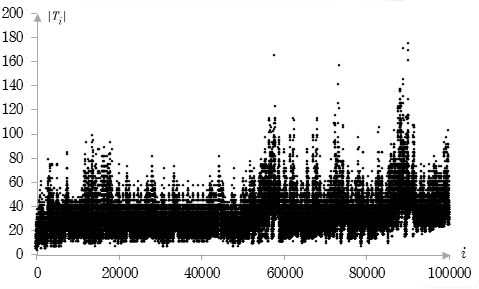
Fig 1. Size of the theorems derived by Program 1.

Attachments

1. The program.
2. Text file with 100 000 derived theorems and their proofs.
3. CSV file with theorems and related data.
4. CSV file with less important details on program execution.

5. Program 2.

Described algorithm can be improved by rejection of instances and addition of preference for a shorter theorems, i.e. standard "best first" strategy.

1. Theorems T₁, T₂, ..., T₁₀ are the axioms of propositional calculus.
2. Theorem T_n+1 , for n = 10, 11, ... is the first theorem such that
   1. it can be derived by single application of the combined rule on pairs of theorems T₁, T₂, ..., T_n,
   2. it is not an instance of any of these theorems, and
   3. there is no shorter theorem satisfying conditions a. and b.
   The theorems are derived by single application of the combined rule on the pairs of the theorems, ordered by Cantor's enumeration.

The program is developed in newLISP and executed for nearly two weeks on few years old personal computer. Application of the combined rule is attempted 10 000 000 001 times. It failed in 51% of attempts because premise major wasn't implication. In 23% of attempts unification of antecendent in premise major and premise minor wasn't possible. In 26% of attempts unification succeeded and conclusion is developed. In 13% of attempts, conclusion was too long to be added to the theory in any reasonable time; it is unknown how many duplicates were among these. Nearly 13% attempts resulted in duplication of already derived theorems. Finally, 0.0065% attempts were successeful and 0.001% attempts resulted with 100 001 shortest theorems. 

Following table contains the list of all theorems of the size (defined as number of operator and variable occurences) less or equal to five, derived by program, with some related data.

For instance, T₃₈₃₈₄, ((not A) or A) has the following proof, as printed out by program:

Notation tm- stands for internal representation of theorems in program. For instance, T₃₈₃₈₄ is tm-203408.

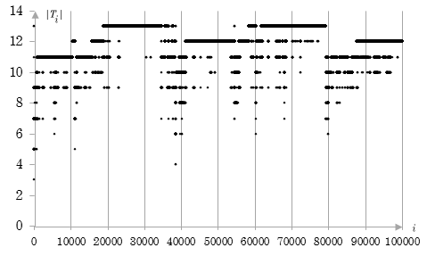
Fig 2. Size of the theorems derived by Program 2.

The graph shows that derived theorems are much shorter than those derived with Program 1. It is clearly visible which theorems are relatively short, yet they are derived relatively lately. Theorems T₃₈₃₈₄ and T₃₈₃₈₅, for instance, are among these. Some short theorems are used in futher derivation of short theorems. It is seen on graph as dent in graph; for instance, between T₃₈₃₈₃ and T₅₄₄₈₂. The width, depth and area of the dent suggest the importance of the theorem a posteriori. It appears that there is a correlation with size of proof as measure of the importance of theorem a priori. 

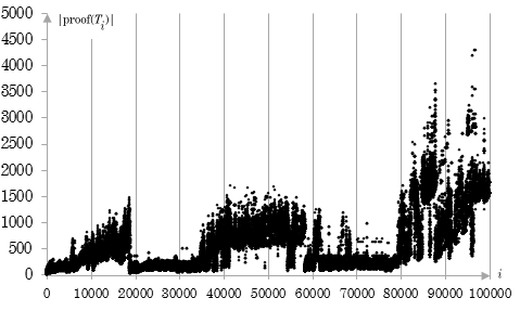
Fig. 3. Size of the proofs of theorems derived by Program 2.

A few weaknesses of Program 2. are obvious. Although derived theorems are not instances of a previously derived theorems, human can recognize that many of these theorems are weak. For instance, theorems containing double negation; theorems of the form (F or G), where at least one of the formulas F and G is a theorem; theorems with subformulas of the form (F or F), (F and F), where F is any formula; thorems that could be obtained by application of commutativity and associativity of operations or and and and so forth.

Attachments

1. The program.
2. Text file with 100 001 derived theorem and their proofs.
3. CSV file with theorems and related data.
4. CSV file with less important details on program execution.

6. Conclusion

The program should be extended to reject more trivial variations of already derived theorems, as humans do. The results obtained so far appear to be interesting enough to justify further experiments.

References

1. Colton, S. and Bundy, A., "On the Notion of Interestingness in Automated Mathematical Discovery" in Proceedings of the AISB'99 Symposium on AI and Scientific Discovery, Edinburgh, UK, 1999.
2. Mendelson, E., Introduction to Mathematical Logic, many editions.
3. Poincare, H., Science and Method, Dover Publications, Mineola, 2003.
4. Wang, H., Toward Mechanical Mathematics, IBM Journal of Research and Development, Vol. 4 No. 1, January 1960, pp. 2-22.
5. Wang, H., Survey of Mathematical Logic, Nort Holland, Amsterdam, 1963.
6. Wos, L., Automated Reasoning: 33 Basic Research Problem, Prentice-Hall, 1988.
7. Wos, L., The Problem of Automated Theorem Finding, Journal of Automated Reasoning, Vol. 10 No. 1, 1993, pp. 137-8.